During my second-grade bachelor's year (2011-2012) we were told that we should start bothering to find a scientific advisor, since (winter) third grade is coming. That was exactly the year when my future scientific advisor visited our branch of university and had given us an astonishing «Introduction to graph theory» course. I was so impressed with this course and with the way how it was presented to us, that did not waste a minute after the last lecture and asked my future scientific advisor to work with me and give me some tasks to work on (luckily he agreed). Since then I never changed a scientific advisor (although had changed research topic once), but it did not work out well with graph theory research, so I continued with automata theory and ended up with a PhD thesis. Still, my warm feelings to graph theory did not vanish and from time to time I'm trying to find some interesting topics from that field to study.

Some time ago I started wondering if it is possible to find something new in a very old and well-known task of planar coloring, especially from an algorithmical viewpoint. I was lucky to get some assistance from my former student Matveeva Asya, who happened to be interested in some mini-research on this topic, and agreed to help me with coding and illustrations.

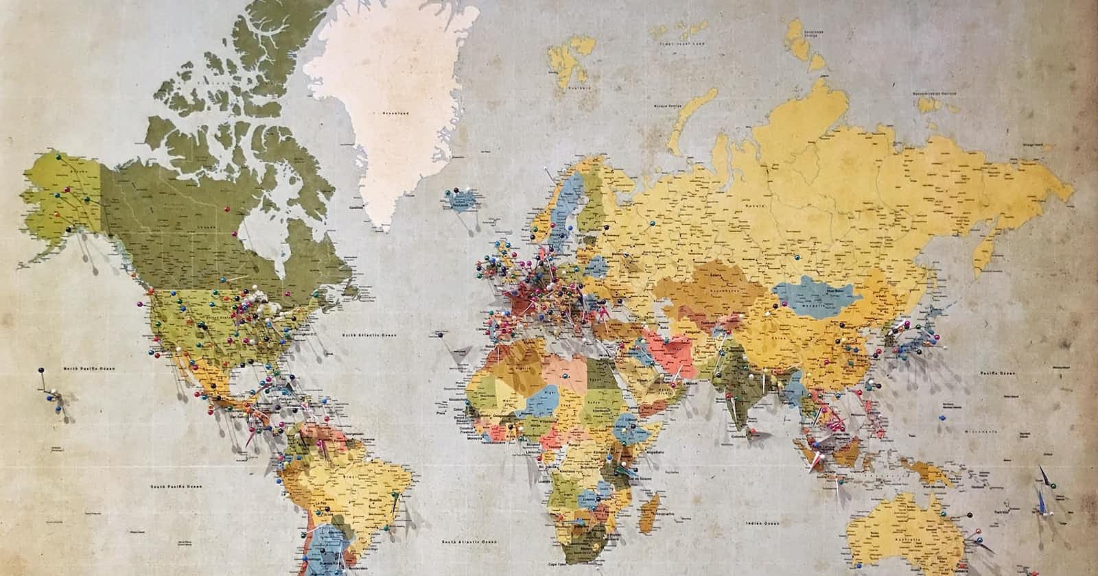
So, if you never happened to stumble upon a planar coloring task from graph theory, the main idea for you can be found in this picture:

From mathematical point of view such maps are just planar graphs (although depicted in a very fancy way) and the task is to perform a graph coloring, i.e. to label each vertex in a graph (on the maps these are just some countries) with different colors, so that each vertex won't have a neighbour with the same color (no two neighboring countries will use the same color). Let's make it a bit more formal:

Graph is a tuple of sets (V,E) where V - set of vertices, E - set of edges on these vertices. Planar graph is a graph that can be pictured on a plane without edges intersections. Graph coloring (correct graph coloring) - is a rule to label vertices with some set of colors C, such that no edge from E connects two vertices with the same label.

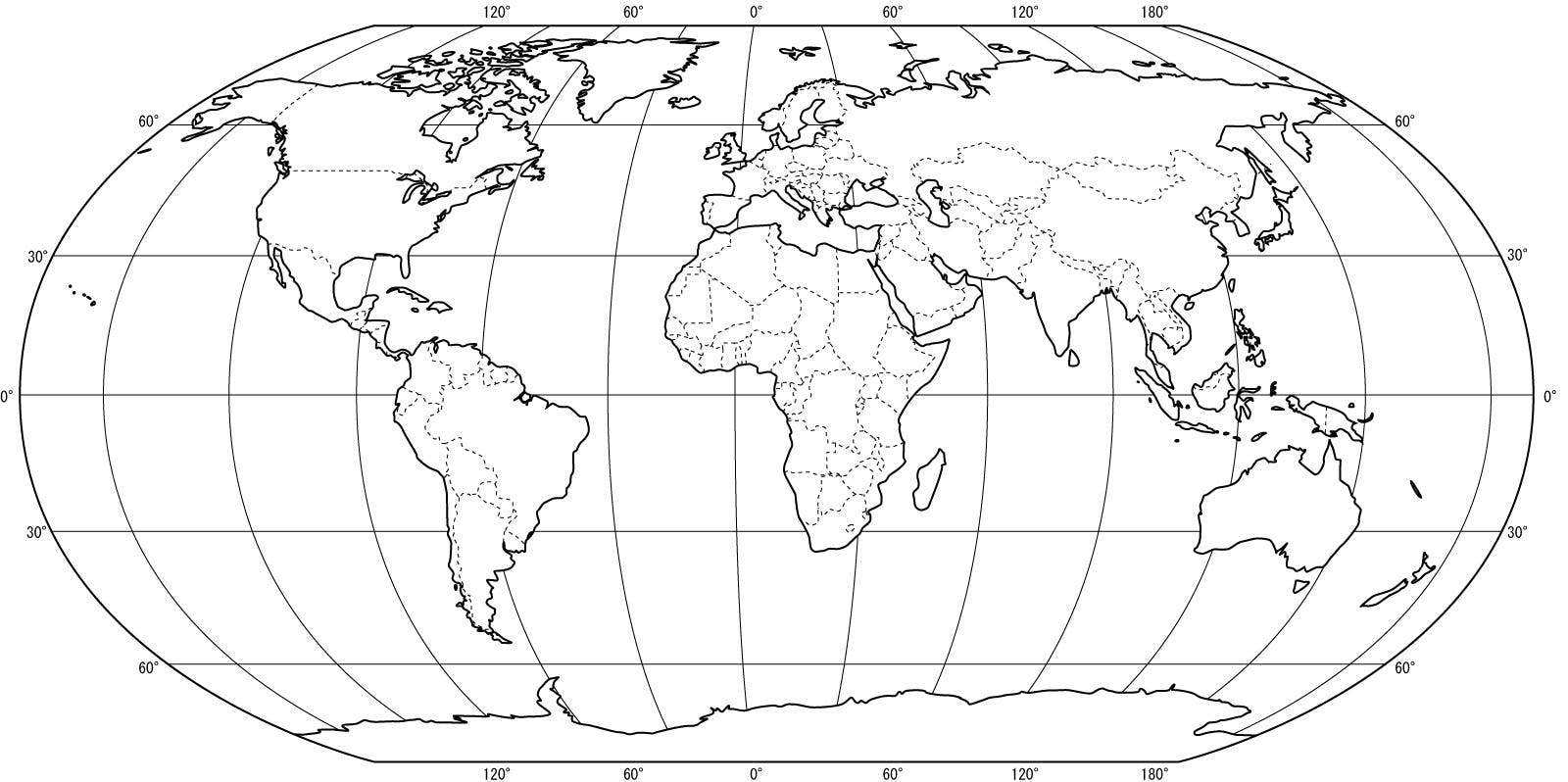
Before we continue with coloring problem, let's think about some graphs that are not planar. In fact there are two most important non-planar graphs which are K5 (full graph on 5 vertices) and K3,3 (bipartite graph with 3 vertices in each part). These two cannot be pictured on a plane without edge-intersection anyways:

They are the main ones since there is a well-known Pontryagin-Kuratowski theorem, which states that these two graphs are appearing as a subgraph of any non-planar graph after a set of specific modifications on a graph (and this is a criteria for non-planar graphs).

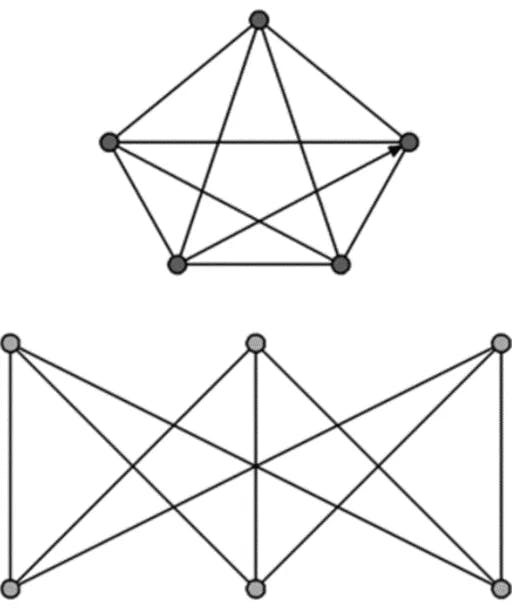
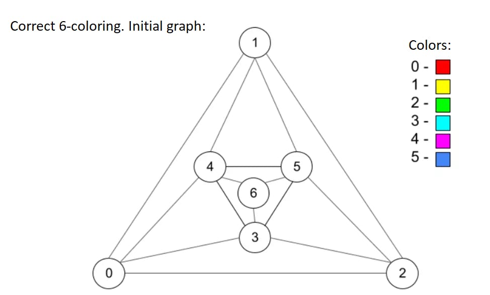
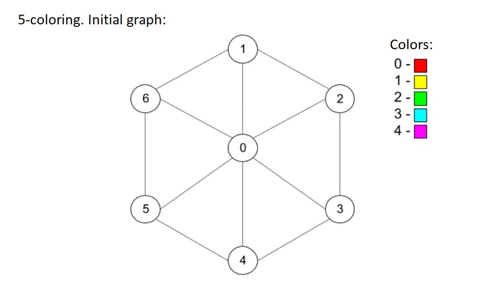
Planar graphs are quite easy to imagine, for example if we think of the map from the first picture in this way: each country is a vertex and all it's neighbors are connected with this vertex through an edge. This graph definately will be possible to draw without edges intersections. But to dive into graph coloring some more, let's look at one example of planar graph with some correct coloring applied:

Here we have six vertices (numbers in circles are vertex numbers), edges are not intersecting (so graph is planar) and coloring is right (no two vertices connected with an edge have the same color).

For any planar graph there is always a right coloring if you take many different colors, but the most interesting task is to find a minimum number of colors required to use for correct coloring — such a number is called a chromatic number. There is a quite famous four color theorem which states that any planar graph can be colored using only 4 colors (and the proof of this theorem brings a lot of controversy). In this article we won't work with this extreme and use a bit more colors (5 and 6) though. One more thing to mention is that this task in fact has a lot of interesting applications, so graph coloring is not useless. Ok, now let's dive into some algorithms.

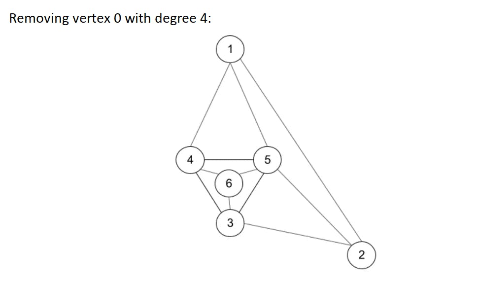
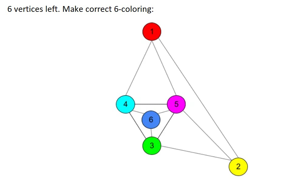
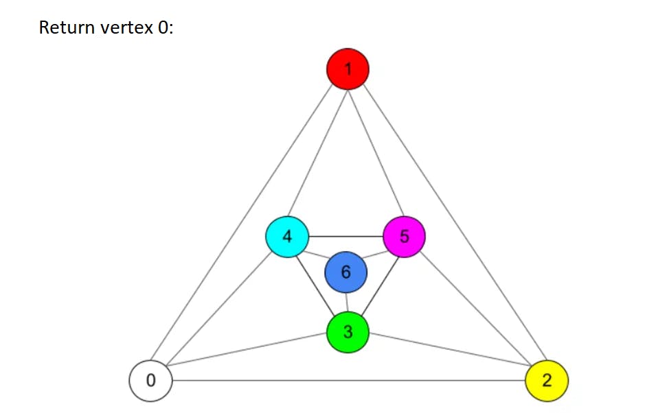
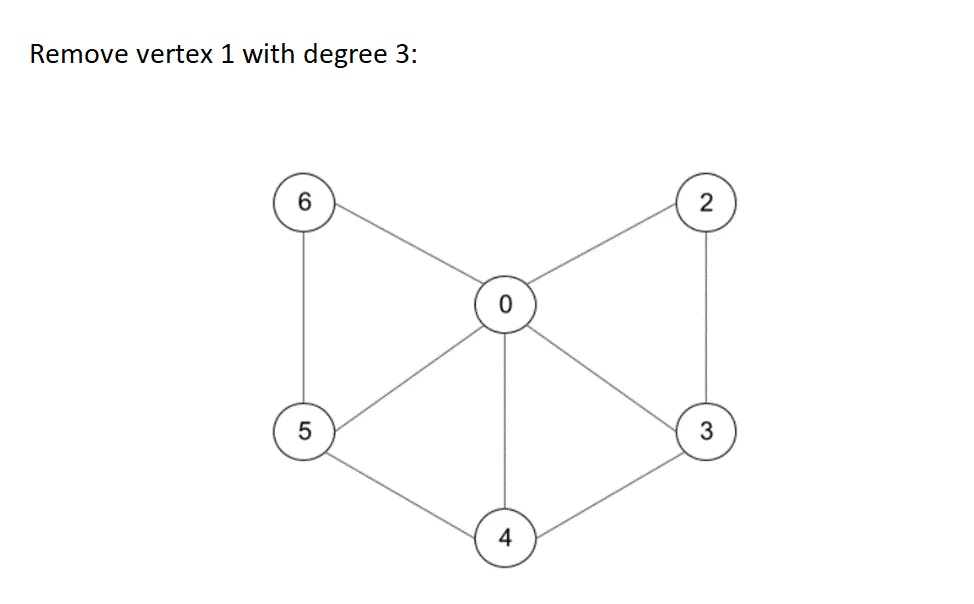
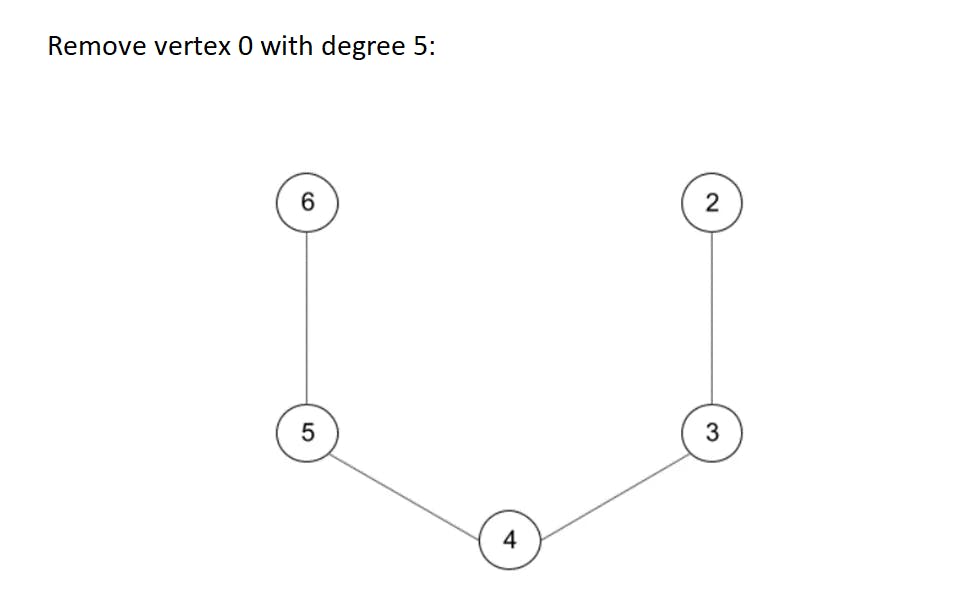
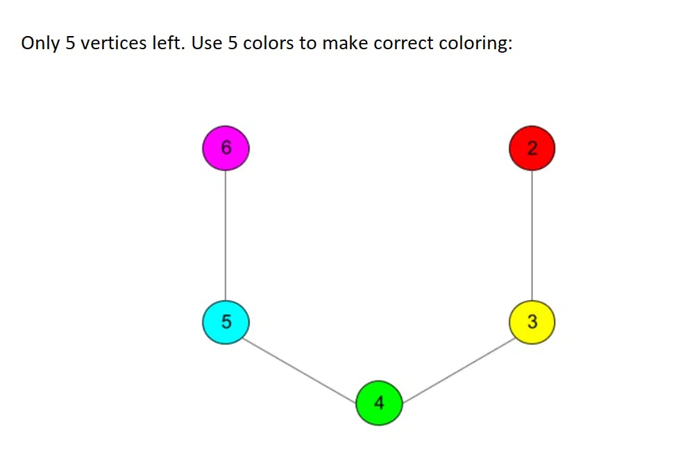
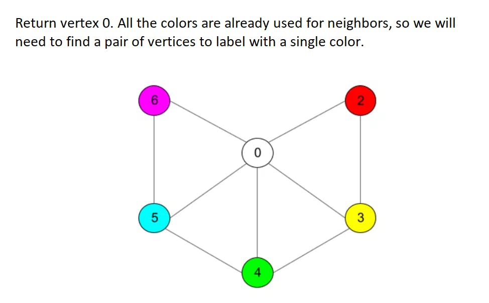
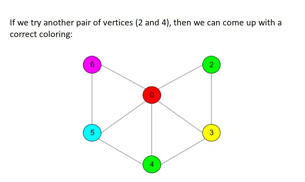
Let's start with a 6-colors theorem, which states that 6 colors are enough to color up any planar graph. The proof is simple, we use Euler's formula to derive the fact than any graph always has a vertex of degree no more than 5 (degree of a vertex is a number of vertex neighbors). If we delete such a vertex from graph (and save this operation in some history log), we will get to another planar graph but with less vertices. If we continue to use this trick many times we will eventually come to the graph with no more than 6 vertices which is easy to color in 6 different colors. Then we have to roll back our history log and return deleted vertices, and color the returned vertices in such a way that 6 colors will be enough for right coloring (this is possible since each deleted vertex had no more than 5 neighbors). Let's look at this algorithm in action on an example graph from the previous picture:

This is a very simple theorem and it gives an exact algorithm to make correct 6-coloring. Let's put it into some code for better understanding:

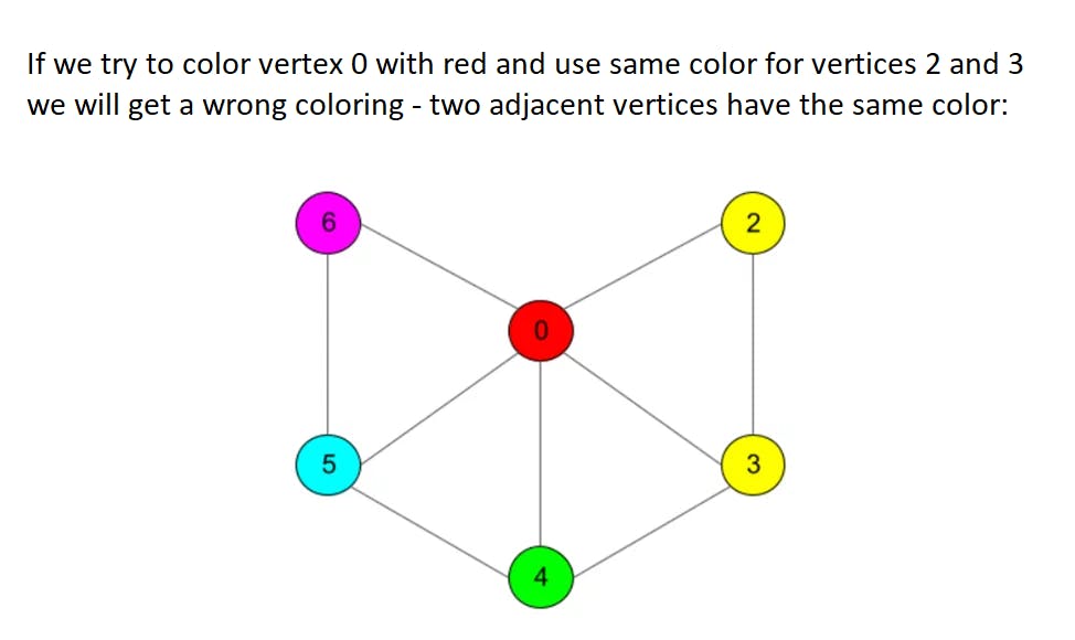
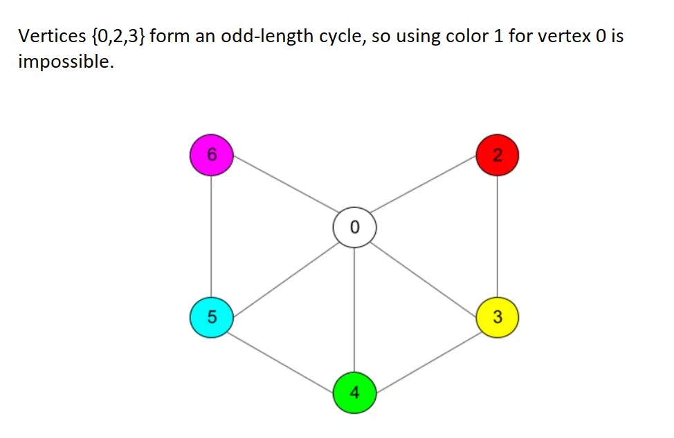
Ok, 6 colors are enough, now we are sure. How about 5? To prove that 5 colors are enough we need a bit more work though. First steps in a proof are quite similar, we will delete vertices with no more than 5 neighbors until our graph is left with no more than 5 vertices to use 5 colors only. When we start returning deleted vertices we will face a problem: some vertex could have 5 neighbors that will appear to be colored in 5 different colors. However, this can be solved with a specific trick: there will always appear two vertices from this neighbors set that can be recolored in a single color (although we will probably need to recolor some chains of vertices to make coloring right). For details plese refer to the full proof while we will work through a simple example here:

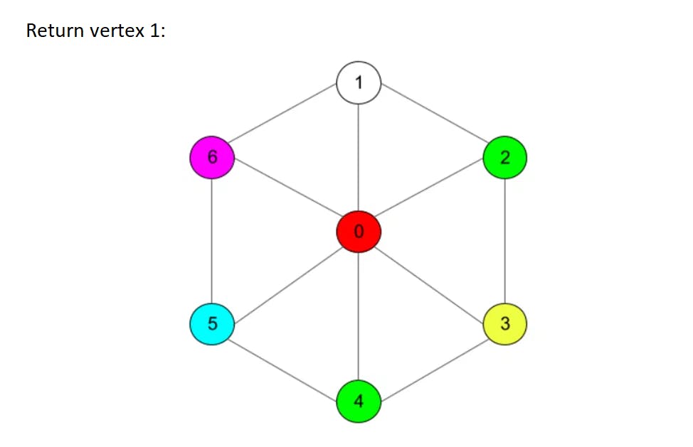
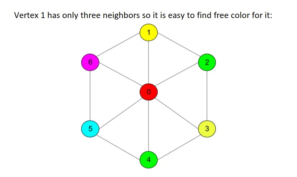
Algorithm now is more complex since we need to «run through» neighbors in search of a chain that can be recolored. For any new vertex added the length of such a chain can grow up to the number of vertices in a graph in the worst case, so asymptotic complexity reaches O(n^2). Take a look at an example listing:

A natural question that now arises is the following: «Can we construct planar 5-coloring faster than in quadratic time?». If the number of vertices in a planar graph is too large we wouldn't like to wait for quadratic algorithm to end.

It turned out that in 1980 there was already found a linear-time algorithm that solves planar 5-coloring problem, but it is not so shiny as it looks like...

In the mentioned article from a group of Japanese researchers there are some hidden matters, if we can say so. Some very specific constraints are not listed in the annotation and many difficulies may arise when reading it through. First of all, for the linear 5-coloring algorithm the authors suppose that they already know a planar embedding of a graph (since it is planar, there is one) and adjacency lists at input are in fact sorted clockwise or counter-clockwise (in correspondence with the planar embedding). Second thing to mention is that these adjacency lists for graph are not so simple — it is supposed by authors that one can remove vertex from list with O(d) time, if d is a degree of a vertex. Similarly it is supposed that merging two vertices with degrees d1 and d2 can be made with O(d1+d2) complexity. In the naive adjacency-lists structure such operations cannot be performed so fast, but we can «model» adjacency lists with hashtables (still we will need to store order of neighbors), so this complexity can be achieved.

It was a bit disspointing that authors of the article did not underline these things and did not mention the constraints in the annotation, but still we figured everything out eventually.

Let's outline the main idea of the article. The proposed method tries to achieve the case that is similar to 6-colors theorem, i.e. when new vertex has no more than 4 different colors neighboring. Authors modify deleting procedure in such a way that instead of just removing vertices with no more than 5 neighbors, they also consider vertices of degree 6, and some of the removed vertices are also merged in process, so that we guarantee the required coloring property when we'll roll back the procedure. To make a good complexity we will try to merge as much vertices as possible in a single step, and the selection of such sets to merge is described in the article in details (and for this we are heavily using the knowledge of planar embedding). Let's finally look at the example listing of O(n) 5-coloring:

This code is demonstation-purposes only, and that is the reason why it uses recursion, so on too-large amount of vertices you can catch stack-overflow. One can get rid of the recursion in this code (simply simulate call-stack in your code).

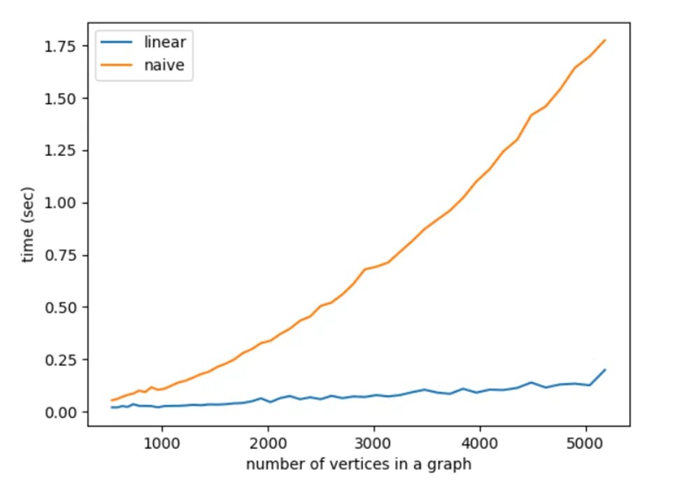
As a cherry on the cake we made an experimental time comparison for the «naive» 5-coloring and linear one. As a test data we use planar graphs, corresponding to Cartesian plane grid of a fixed size. Here are the graphs of speed for 10 runs on each fixed graph size:

That's all for today. I would like to give again my thanks to wonderful Matveeva Asya and wish her all the best in future work!

Thank you for reading this article, stay tuned for new beautiful algorithms. Subscribe for new articles and share your reactions if you liked this material.

Wish you all the best and a trully colorful life (with the number of colors far beyond planar chromatic number)!