


Geometry is beautiful and hard at the same time. At school, I enjoyed it a lot, but then lost interest during my university studies. Eventually, I returned to geometry when I started working as a Math teacher at school. It so happened that I had to recall all my knowledge quickly for the teacher’s work, and, although school material is not too complex, it was quite challenging for me (I’m just not the brightest one, you know). Still, this preparation work brought me a lot of pleasure, since the beauty of geometry cannot leave a mathematician ignorant. It was exactly this time when I met Asya Matveeva at the mentioned here school. Asya is a very talented student who is not only truly interested in science but also has wonderful research and programming skills. She proposed to write one more article together, and I was quite delighted to agree, of course. You can check out our previous common article here, today let’s dive into some triangulation tasks.
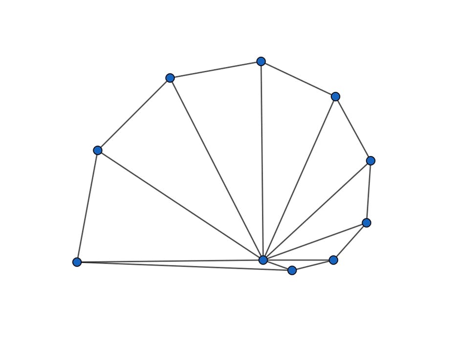
Triangulation is (simply speaking) a way to draw triangles “on top” of the given set of points on the plane (we will work on Euclidean 2D plane only) so that the vertices of triangles are drawn from the set of points, edges do not intersect anywhere apart from these vertices, and some points may be on the same edge of some triangle. If we required that no more than two points lie on the same line, there would not be a case when more than 2 points lie on the same edge, but let’s consider all the possibilities. Take a look at the following picture with a triangulation example:
It is not too hard to understand that the triangulation for a given set of points exists almost always, except for the degenerate case when all the points lie on the same line. Moreover, at first glance it may appear that building a triangulation is quite an easy task (and it is, but maybe not as easy as you think), but sometimes it is interesting to build not just any triangulation on the given set of points but a “good” one. What on earth could it take for triangulation to be “good”?
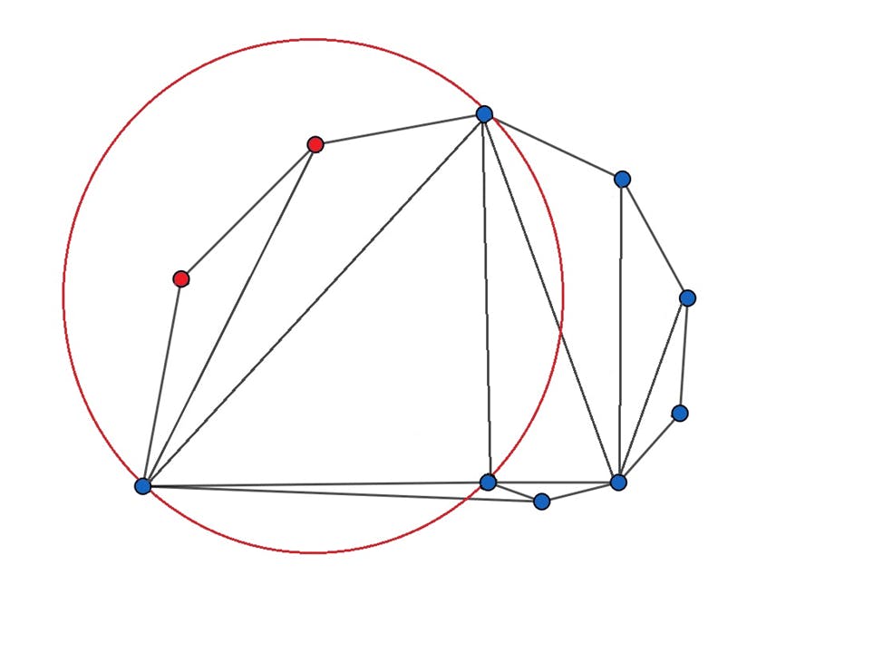
There is a very beautiful class of Delaunay triangulations such triangulations that for any triangle in the triangulation and a circumcircle of this triangle, there would be no points inside the circumcircle. It may be hard to grasp the definition at once so just look at the following pictures where you can see examples of both not-Delaunay (first picture) and Delaunay (second one) triangulations:

So why are such triangulations “good”? From the applications which we will mention at the end of this article you will understand it better, but for now, maybe it would be useful to know that such triangulations are tightly connected with Voronoi diagrams which are used in the extremely large variety of applications (check out the wiki page for more details).
What we would like to do is to understand how fast we can search for the Delaunay triangulation for the given set of points as input. The most naïve way to do it is just to look through all the possible triangulations that can be constructed and choose the one that satisfies Delaunay's property (which is – that no point lies inside a circle around any triangle). Quite obvious that this approach is not just complex, but extremely complex – searching through all the possible triangles to build a triangulation would take exponential time.
The first task for Asya was to come up with some algorithm that is polynomial in time and allows to build a Delaunay triangulation if one exists. She successfully found a simple way, which is used in some of the well-known Delaunay triangulation algorithms. Let’s first describe her idea:
Suppose we somehow have built the first triangle which is sure to appear in some Delaunay triangulation (yes, Delaunay triangulation may sometimes be not unique for a given set of points – consider this statement a small exercise to think about). To build the next triangle we will consider an edge of the already found triangulation and look through all the points which are:
Not in the triangulation yet;
Appear in the half-plane which is different from the one where the third point for a triangle, from which we took the current edge, lies.
Among all these points we will select the ones that have the biggest angle from which the current edge is seen (i.e. if the edge is made of the segment on points A and B and we select some candidate point C, we suppose the angle ACB is the biggest among all the other candidate-points C’). If such a point is a single one, we just build a new triangle with the current edge and a new point and add two new edges which we’ve built to some edge-candidate queue (from which we will take the next edges for consideration). If there were several such points we will select them all, get a convex polygon in which all the points lie on the same circle (say hello to school geometry here), and construct a triangulation for such a polygon in a special way.
This procedure will continue until all the points are used in some triangle. The only thing we did not describe yet is how to select the first triangle for the triangulation to start. Here we will just do a simple trick – we will take the leftmost point by x coordinate and select a line with the largest absolute slope value which goes through this point and some other points. There could be some corner cases if such a line is not unique – we will just process them manually. For the constructed line we simply find the point for triangulation in the same way we described before.
Before we go to the code let’s consider the illustrative example of the described algorithm (the process is illustrated from left to right, from top to bottom):
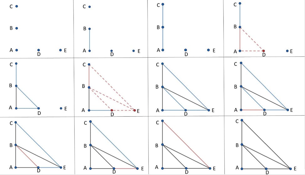
Light blue lines in this illustration are the candidate edges that were added to the queue for further consideration (to continue building the triangulation), and black ones are the lines that are out of the queue or have never been added to the queue because they had already had the necessary amount of neighbors (from left and right half planes), and red lines are the candidates under consideration at the current step. The red dotted line is the candidate to be added to the queue, and the red solid line is the current candidate edge in consideration. In this illustration, B, C, D, and E all lie on the same circle, which is why when the edge BC is under consideration we add several edges to the queue (BD, CE, DE) for proper triangulation.
It is not hard to prove that such an algorithm is correct and that its complexity would be O(N^2) where N is the number of points (but from the code, it would be obvious). You can look through the code in Python which embodies the described procedure:
import math
import random
from turtle import *


#returns the cosine of an angle at which an edge is visible from a given point
def cos(edge, point):
    pe1 = [edge[0][0] - point[0], edge[0][1] - point[1]]
    pe2 = [edge[1][0] - point[0], edge[1][1] - point[1]]
    return round((pe1[0] * pe2[0] + pe1[1] * pe2[1])/math.dist(edge[0], point)/math.dist(edge[1], point), 14)


#returns the sine of an angle at which an edge is visible from a given point
def sin(edge, point):
    pe1 = [edge[0][0] - point[0], edge[0][1] - point[1]]
    pe2 = [edge[1][0] - point[0], edge[1][1] - point[1]]
    return round(abs(pe1[1] * pe2[0] - pe1[0] * pe2[1])/math.dist(edge[0], point)/math.dist(edge[1], point), 14)


#returns the coefficients of a line (a * x + b * y + c = 0) through two given points
def line(p1, p2):
    a = p1[1] - p2[1]
    b = p2[0] - p1[0]
    c = p1[0] * p2[1] - p2[0] * p1[1]
    return [a, b, c]


points = []
for i in range(7):
    x = random.randint(-5, 5)
    y = random.randint(-5, 5)
    points.append((x, y))
points = list(set(points))
points.sort()
p0 = points[0]
edges = [] #queue with edges
triangulation = {}  #dictionary with edges as keys, and points connected to them as values


#First step is to find a line throw p0 and another point from points with the greatest absolute value of slope possible. Every two adjacent points from points[] on the line give a new edge in triangulation. For n points there will be (n-1) edges.
max_abs_slope = [0]
for point in points[1:]:
    if point[0] == p0[0]: #Since the slope of a vertical line is undefined as the denominator is equal to zero, it is represented as an infinite value.
        slope = float('inf')
    else:
        slope = (point[1] - p0[1])/(point[0]-p0[0])
    if abs(slope) > abs(max_abs_slope[0]):
        max_abs_slope = [slope, point]
    elif slope == max_abs_slope[0]:
        max_abs_slope.append(point)
max_abs_slope[0] = p0
for i in range(1, len(max_abs_slope)):
    new_edge = tuple([max_abs_slope[i-1], max_abs_slope[i]])
    edges.append(new_edge)
    triangulation[new_edge] = []


#Second step is to find the point from which an edge is visible at the greatest angle for every edge in edges[]. Since every edge in edges[] is already connected to a point (except for the edges added in the beginning of the algorithm), the new point is searched in a different half-plane.
while len(edges) > 0:
    edge = edges.pop(0)
    if len(triangulation[edge]) == 2:
        continue
    coeff = line(edge[0], edge[1])
    a, b, c = coeff[0], coeff[1], coeff[2]
    if len(triangulation[edge]) == 0:
        fixed_point = [edge[0][0] - 1, edge[0][1]]
    else:
        fixed_point = triangulation[edge][0]
    fixed_dist = a * fixed_point[0] + b * fixed_point[1] + c
    vertex = [2, []]
    for point in points:
        if (a * point[0] + b * point[1] + c) * fixed_dist < 0: #fixed_point and new point are in different half-planes in relation to the edge
            cosine = cos(edge, point)
            angle = cos((edge[1], point), edge[0])
            if cosine < vertex[0]:
                vertex[0] = cosine
                vertex[1] = [[angle, point]]
            elif cosine == vertex[0]:
                vertex[1].append([angle, point])
    if vertex[0] != 2: #vertex[0] == 2 in case of the absence of points in the half-plane
        on_circle = vertex[1][::] #this list contains the vertices of the inscribed polygon except edge[0] and edge[1].
        on_circle.sort()
        on_circle.append([1, edge[1]])
        triangulation[edge].append(on_circle[0][1])
        new_edge = tuple(sorted([edge[0], on_circle[0][1]]))
        if new_edge not in triangulation.keys(): #new_edge is not connected to any points yet.
            triangulation[new_edge] = [on_circle[1][1]]
            edges.append(new_edge) #new_edge is added to the queue because one more point could still be connected to this edge.
        elif on_circle[1][1] not in triangulation[new_edge]: #connect new_edge to on_circle[1][1], if this has not been done already.
            triangulation[new_edge].append(on_circle[1][1]) #new_edge is not added to the queue because it is already connected to two points.
        for i in range(len(on_circle)-1): #building outer edges of the inscribed polygon.
            new_edge = tuple(sorted([on_circle[i][1], on_circle[i+1][1]]))
            if new_edge not in triangulation.keys(): #the same check as for the previous new_edge
                triangulation[new_edge] = [edge[0]]
                edges.append(new_edge)
            elif edge[0] not in triangulation[new_edge]:
                triangulation[new_edge].append(edge[0])
        for i in range(1, len(on_circle)-1): #building inner edges of the inscribed polygon.
            new_edge =  tuple(sorted([edge[0], on_circle[i][1]]))
            triangulation[new_edge] = [on_circle[i-1][1], on_circle[i+1][1]]


for key, val in triangulation.items():
    print(key, ":", val)


def rendering(points, triangulation, k):
    speed(1000)
    up()
    color("red")
    for point in points:
        goto(point[0] * k, point[1] * k)
        dot(5)
        up()
    color("black")
    for key in triangulation.keys():
        goto(key[0][0] * k, key[0][1] * k)
        down()
        goto(key[1][0] * k, key[1][1] * k)
        up()
    exitonclick()


rendering(points, triangulation, 30)
All right, we’ve got our first algorithm working, now it is time to come up with a better procedure because N^2 seems a bit too much when the number of points becomes larger. Here we decided to search for some knowledge online and found this very useful article (it is in Russian, but I think auto-translators will easily handle it). The author of this article, Pavel Kositsyn, proposed a very neat pipeline based on the sweep-line procedure for the construction of Delaunay triangulation. Here’s the basic idea of the algorithm:
All the points are sorted by x coordinate (just as we did already)
Build the first triangle on the first three points. The algorithm always preserves the property that the currently constructed triangulation is Delaunay and we always keep the min convex hull for the constructed part.
Pick the next point in the cycle which is not in triangulation yet. Using the sweep-line approach construct a visibility graph for this point and all the points from the already-constructed convex hull. Connect all the points which are in this graph and are visible from the currently selected point.
For the newly constructed bunch of line segments check if all the quadrilaterals, which appeared due to these new segments, are holding the Delaunay property. If some of them are not Delaunay, we simply switch edges in this quadrilateral and go recursively by the edges of this quadrilateral to fix all the possible non-Delaunay constructions which could appear due to this change.
In this algorithm, on average we optimize the number of points under consideration when we add new triangles to the currently constructed triangulation. To get a better understanding of the algorithm take a quick look at the following picture which shows the example of the algorithm flow (once again, from left to right, from top to bottom):
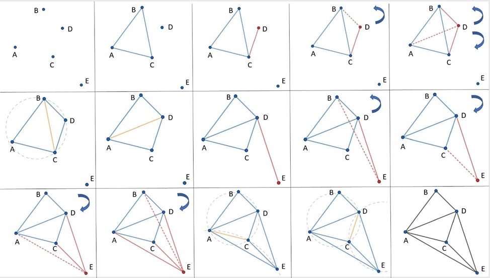
Here we first construct triangle ABC after sorting, and adding A<->C<->B to the convex hull (counterclockwise). We pick a point D, since C has the largest x coordinate it is visible to D and DC does not intersect with any other edge. We start moving sweeping line counterclockwise to select visible points and soon enough we see that only B and C are visible (for this we use the cross product of vectors). We add D to triangulation and check the Delaunay property for all constructed quadrilaterals. Unfortunately, it does not hold in the current triangulation, so we switch the edge BC to AD, and then the Delaunay property starts holding. We modify our convex hull to A<->C<->D<->B. Then we peek at point E, and start searching for visible points first counterclockwise, then clockwise (when we stumble upon invisible points). We add edges EA, EC, ED, since these three points are visible, and check Delaunay property for the whole construction.
The author hypothesizes that the presented algorithm works in O(N*logN) time on average, which seems to be quite a reasonable assumption (of course, not in the worst case).
The main challenge of this task for Asya was to write this algorithm herself, in Python, thus she had to clearly understand all the steps and data structures required for the fast search of candidate points. The good thing is that she could always check some C++ code of the author’s solution for reference (thanks to Pavel Kositsyn). For the reader, it could also be a good challenge to work through such a task on your own, but if you would simply like to see how we embodied this algorithm, please refer to the following code:
import math
import random
from turtle import *


#returns the cosine of an angle at which an edge is visible from a given point
def cos(edge, point):
    pe1 = [edge[0][0] - point[0], edge[0][1] - point[1]]
    pe2 = [edge[1][0] - point[0], edge[1][1] - point[1]]
    return round((pe1[0] * pe2[0] + pe1[1] * pe2[1])/math.dist(edge[0], point)/math.dist(edge[1], point), 14)


#returns the sine of an angle at which an edge is visible from a given point
def sin(edge, point):
    pe1 = [edge[0][0] - point[0], edge[0][1] - point[1]]
    pe2 = [edge[1][0] - point[0], edge[1][1] - point[1]]
    return round(abs(pe1[1] * pe2[0] - pe1[0] * pe2[1])/math.dist(edge[0], point)/math.dist(edge[1], point), 14)


#checks if the triangulation of four points is a delaunay triangulation
def delaunay_correct(edge, p1, p2):
    sin1 = sin(edge, p1)
    cos1 = cos(edge, p1)
    sin2 = sin(edge, p2)
    cos2 = cos(edge, p2)
    return sin1 * cos2 + sin2 * cos1 >= 0


def cross_product(vector1, vector2):
    x1, y1 = vector1[1][0] - vector1[0][0], vector1[1][1] - vector1[0][1]
    x2, y2 = vector2[1][0] - vector2[0][0], vector2[1][1] - vector2[0][1]
    return x1 * y2 - x2 * y1


points = []
for i in range(6):
    x = random.randint(-7, 7)
    y = random.randint(-7, 7)
    points.append((x, y))
points = list(set(points))
points.sort()
triangulation = {}
convex_hull = {}
p0, p1, p2 = points[0], points[1], points[2]
convex_hull[p1] = [p0]
triangulation[(p0, p1)] = []
prev = p1
s = 2
#building either a triangle, or (in case first three points are on the same line) a line through first three points
while s < len(points) and (p1[1] - p0[1]) * (points[s][0] - p0[0]) == (points[s][1] - p0[1]) * (p1[0] - p0[0]):
    triangulation[(prev, points[s])] = []
    convex_hull[prev].append(points[s])
    convex_hull[points[s]] = [prev]
    prev = points[s]
    s += 1
if s == 2: #if this is true, first three points are not on the same line
    triangulation[(p0, p1)] = [p2]
    triangulation[(p0, p2)] = [p1]
    triangulation[(p1, p2)] = [p0]
    if cross_product((p2, p0), (p1, p0)) > 0:
        convex_hull[p0] = [p1, p2]
        convex_hull[p1] = [p2, p0]
        convex_hull[p2] = [p0, p1]
    else:
        convex_hull[p0] = [p2, p1]
        convex_hull[p1] = [p0, p2]
        convex_hull[p2] = [p1, p0]
    s += 1
else: #the case in which first n points for n > 2 are on the same line is processed separately
    convex_hull[p0] = [points[s-1], p1]
    convex_hull[points[s-1]].append(p0)
    if s < len(points):
        if cross_product((points[s], p0), (points[s], p1)) < 0: #points[s] is above the line
            for key, val in convex_hull.items():
                convex_hull[key] = val[::-1]
            convex_hull[points[s]] = [p0, points[s-1]]
            convex_hull[p0][1] = points[s]
            convex_hull[points[s-1]][0] = points[s]
        else: #points[s] is below the line
            convex_hull[points[s]] = [points[s-1], p0]
            convex_hull[p0][0] = points[s]
            convex_hull[points[s-1]][1] = points[s]
        edge1, edge2 = (p0, points[s]), (points[s-1], points[s])
        triangulation[edge1] = [p1]
        triangulation[edge2] = [points[s-2]]
        for j in range(1, s - 1):
            triangulation[(points[j], points[s])] = [points[j-1], points[j+1]]
        for k in range(1, s):
            triangulation[(points[k-1], points[k])].append(points[s])
    s += 1


for i in range(s, len(points)):
    point = points[i]
    visible_points = [points[i-1]]
    last = points[i-1]
    right = convex_hull[last][1]
    #finding visible points counterclockwise
    while right != point and cross_product((last, point), (right, point)) < 0:
        visible_points.append(right)
        last, right = right, convex_hull[right][1]
    last = points[i-1]
    left = convex_hull[last][0]
    #finding visible points while moving clockwise
    while left != point and cross_product((last, point), (left, point)) > 0:
        visible_points = [left] + visible_points[::]
        last, left = left, convex_hull[left][0]
    #update convex_hull
    for elem in visible_points[1:-1]:
        convex_hull.pop(elem)
    convex_hull[visible_points[0]][1] = point
    convex_hull[visible_points[-1]][0] = point
    convex_hull[point] = [visible_points[0], visible_points[-1]]
    #add new edges
    edge1, edge2 = tuple(sorted([visible_points[0], point])), tuple(sorted([visible_points[-1], point]))
    triangulation[edge1] = [visible_points[1]]
    triangulation[edge2] = [visible_points[-2]]
    for j in range(1, len(visible_points) - 1): #building edges that connect current point and visible points.
        triangulation[tuple(sorted([visible_points[j], point]))] = [visible_points[j-1], visible_points[j+1]]
    for k in range(1, len(visible_points)): #building visible edges.
        edge = tuple(sorted([visible_points[k-1], visible_points[k]]))
        triangulation[edge].append(point)
        edges = [[edge, point]] #the edges of the polygon connected to the point stored in the sublist do not require rebuilding.
        #sequential rebuilding of the edges
        while len(edges) > 0:
            cur = edges.pop(0)
            cur_edge = cur[0]
            if len(triangulation[cur_edge]) == 2 and not delaunay_correct(cur_edge, triangulation[cur_edge][0], triangulation[cur_edge][1]):
                e1, e2, p1 = cur_edge[0], cur_edge[1], cur[1]
                if triangulation[cur_edge][0] == p1: #edges connected to p1 do not require rebuilding.
                    p2 = triangulation[cur_edge][1]
                else:
                    p2 = triangulation[cur_edge][0]
                #flipping edges
                triangulation[tuple(sorted([p1, p2]))] = [e1, e2] #edge through two points which cur_edge does not contain is added.
                triangulation.pop(cur_edge) #cur_edge is removed
                #since the diagonal in the polygon is changed each outer edge is being connected to another vertex of the polygon.
                triangulation[tuple(sorted([e1, p2]))].remove(e2)
                triangulation[tuple(sorted([e1, p2]))].append(p1)
                triangulation[tuple(sorted([e1, p1]))].remove(e2)
                triangulation[tuple(sorted([e1, p1]))].append(p2)
                triangulation[tuple(sorted([e2, p1]))].remove(e1)
                triangulation[tuple(sorted([e2, p1]))].append(p2)
                triangulation[tuple(sorted([e2, p2]))].remove(e1)
                triangulation[tuple(sorted([e2, p2]))].append(p1)
                #edges not connected to p2 might need to be rebuilt
                edges.append([tuple(sorted([e1, p2])), p1])
                edges.append([tuple(sorted([e2, p2])), p1])


for key, val in triangulation.items():
    print(key, ":", val)


def rendering(points, triangulation, k):
    speed(1000)
    up()
    color("red")
    for point in points:
        goto(point[0] * k, point[1] * k)
        dot(5)
        up()
    color("black")
    for key in triangulation.keys():
        goto(key[0][0] * k, key[0][1] * k)
        down()
        goto(key[1][0] * k, key[1][1] * k)
        up()
    exitonclick()


rendering(points, triangulation, 30)
Ok, it should be faster than our first naïve approach. But how much faster? As we already did in the previous article about graph coloring, we decided to empirically compare the speed of two algorithms and just enjoy some performance charts. Take a look at the charts with different numbers of points and different steps (10, 100, 100, respectively) for testing (and you can also check out correctness and performance tests for the naive and sweep-line approaches):

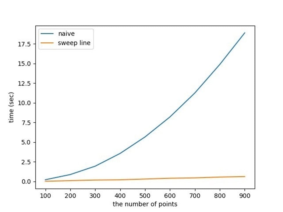

The Naïve algorithm is for sure much slower and it looks quadratic, while the sweep-line is closer to O(N) on these pictures, since it’s time to complete is too little.
Now, when we’ve already done such a great job, why not have some fun? Asya has come up with a wonderful gamification of Delaunay, just to brighten up these boring triangles. She has built up a Python tool with which you can select a photo and put some points on the picture and the program will build and visualize Delaunay triangulation for the selected set of points. Check out some cool triangulated cats, created with this tool:


The source code for this gem (which uses PyGame to work) you can find right here.
To finish with this interesting and not-so-easy topic we should point out some of the applications for Delaunay triangulation. As we have already mentioned, these triangulations are tightly connected to Voronoi cells, which may help to construct an approximation of the shortest path even for the task with obstacles (for example, you can check this article for some intuition about it). Delaunay triangulation is helpful to find Euclidean distance minimum spanning trees which is also a very neat application for network constructions and clustering. They can be used as meshes for some physical modeling tasks in the finite element method. This list is by no means full, you can check out the wiki page that was already mentioned here or search for some cool scientific articles out there – you will surely find a great many of them.
At the very end of this brief note on Delaunay, I would like to give once again many thanks to Asya Matveeva who conducted great academic research on the topic, dived into triangulations, came up with some good algorithms to solve the task, and also built a great entertaining tool to triangulate anything your heart could desire (like cats).
Feel free to like and comment on this material if you found it useful and we will catch up later with some more fun and interesting mathematical and algorithmic topic in this blog. Wish you all the best and send you one final Delaunay triangulation for good luck!
